


1 Gallery
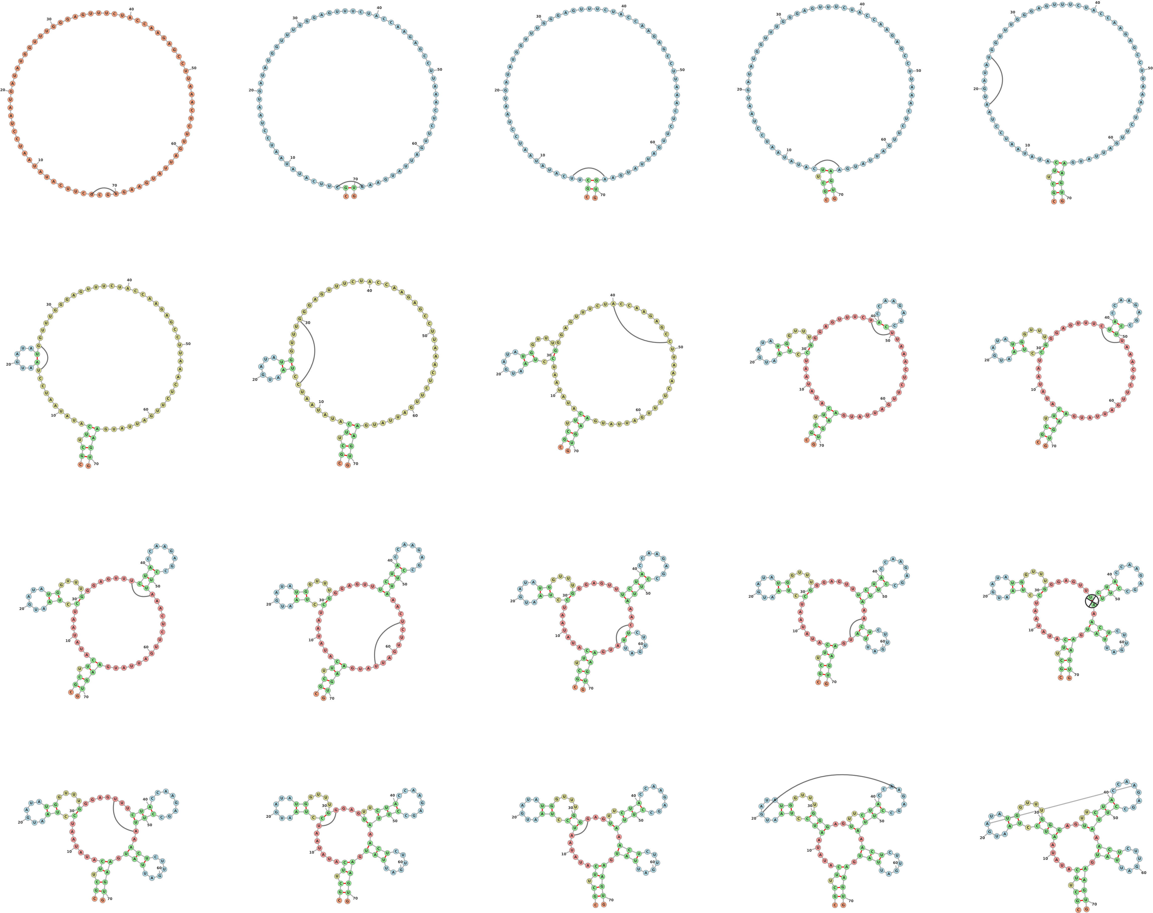
1.1 Drawing a Secondary Structure Starting from an Open Configuration (Figure 1)
One of forna’s key features is the ability to intuitively edit an RNA structure. Links
between unpaired nucleotides are added by holding the shift key and dragging from
one unpaired nucleotide to another. The structure is immediately updated along with
the coloring. The recalculation is performed on the client ensuring lag-free updates.
Unwanted links can be removed by holding ’shift’ and clicking on them. If the user
introduces a pseudoknot with new link, it is detected and added as a force-less
link.
                  >molecule_name

CGCUUCAUAUAAUCCUAAUGAUAUGGUUUGGGAGUUUCUACCAAGAGCCUUAAACUCUUGAUUAUGAAGUG

.......................................................................
1.2 Visualizing a PDB File
PDB files store information about the 3D positions of each atom in a molecule as determined by structural biology methods such as X-Ray crystallography or NMR. While packed with information, they can be difficult to interpret without in-depth knowledge of the structure in question. Extracting the secondary structure requires the use of intermediate programs such as MC-Annotate [1 ]. More recently, RNApdbee [2 ] has been developed as a web service to extract and display secondary structure from PDB files. The resulting images, however, are static and wedded to the layout provided by the visualization tool as well as the secondary structure present in the PDB file.
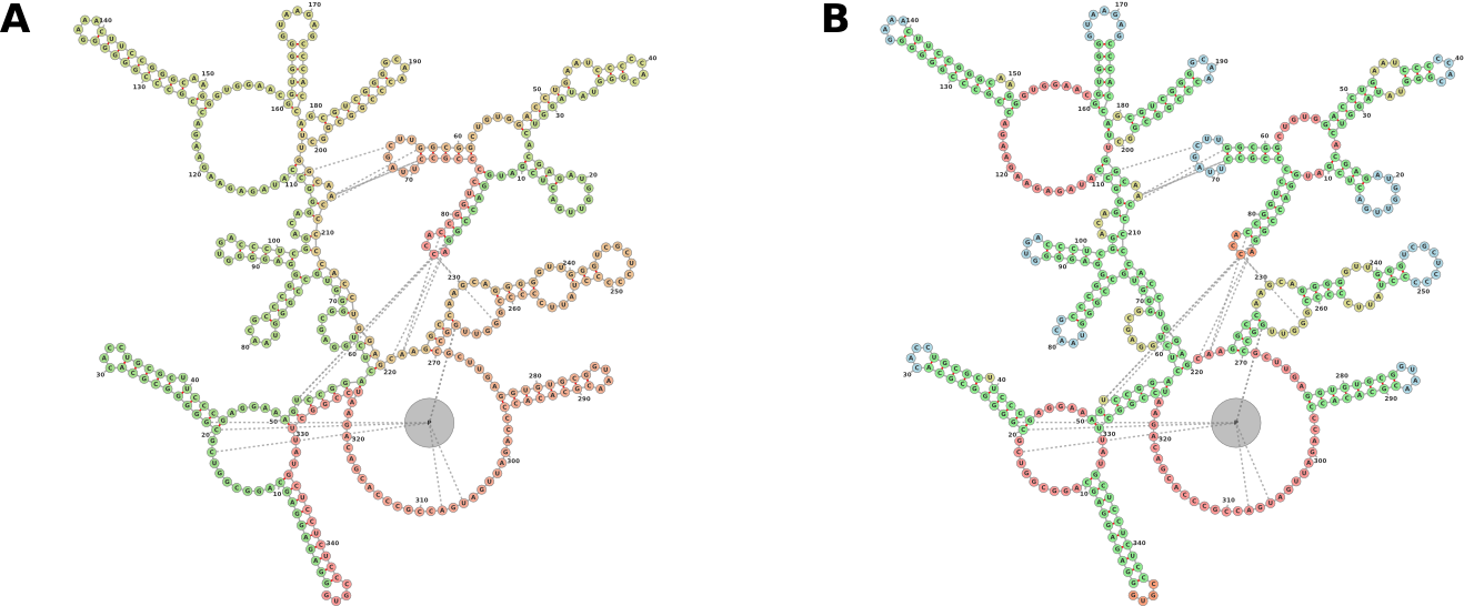
forna extends this functionality by allowing users to input a PDB file and displaying an interactive representation that can be explored and manipulated. Furthermore, forna includes information about protein interactions (an interaction in this case denoting the presence of a nucleotide and an amino acid within 2.8 Å of each other). Figure 2 displays the visualization of a Bacterial Ribonuclease P Holoenzyme in Complex with a tRNA. Immediately evident are the interactions between the ribozyme and the 5’ and 3’ ends of the tRNA as well as the TΨC loop. A protein is seen interacting with the large junction and one of the interior loops of the ribozyme.
1.3 Probing Data
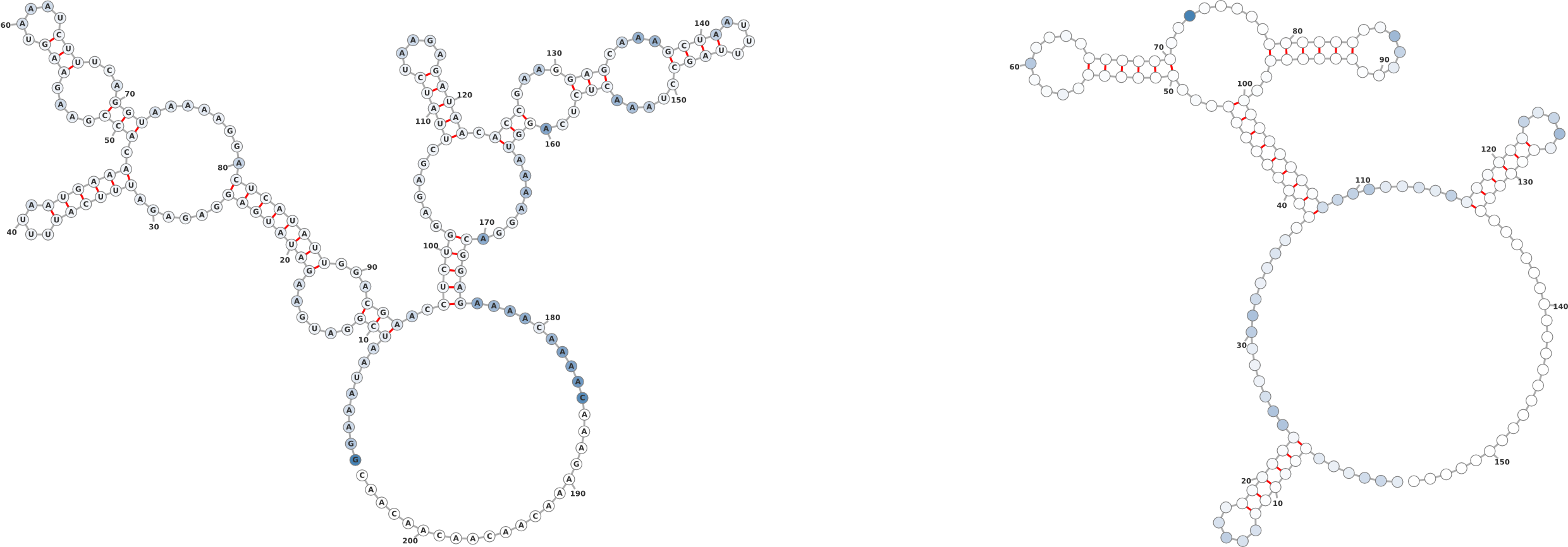
Overlaying chemical probing data on a secondary structure gives researchers an
informative perspective of where highly reactive regions lie. In the examples in Figure
3, it is clear that the probing data is consistent with the given secondary
structure insofar as the highly reactive regions are unpaired whereas the
paired regions exhibit lower reactivity. The example serves to showcase the
ease with which probing data can be overlayed onto a given structure. The
input sequence and structure for the molecule on the left of Figure 3 are as
follows:
                  >GLYCFN_KNK_0002.rdat

ggaaauaaUCGGAUGAAGAUAUGAGGAGAGAUUUCAUUUUAAUGAAACACCGAAGAAGUAAAUCUUUCAGG

UAAAAAGGACUCAUAUUGGACGAACCUCUGGAGAGCUUAUCUAAGAGAUAACACCGAAGGAGCAAAGCUAA

UUUUAGCCUAAACUCUCAGGUAAAAGGACGGAGaaaacaaaacaaagaaacaacaacaacaac

........(((......((((((((......((((((....)))))).(((....(((.....)))...))

)........))))))))...)))..(((((......(((((.....))))).(((....(((....((((.

...)))).....)))...))).......)))))..............................
The probing data was added by clicking on the ’Colors’ drop-up and then on the
’Set’ button. The following values (obtained from the RNA Mapping Database
http://rmdb.stanford.edu/repository/detail/GLYCFN_KNK_0002) were pasted
into the field.
                  247.6424 96.2278 54.8271 46.8534 64.6265 21.8767 39.5119 43.1716 14.4877

8.8179 2.8988 3.7053 23.1721 5.0993 3.4704 49.9487 37.8422 6.636 0.6161

0.3902 13.7014 2.9549 -0.376 1.0762 -0.5679 -0.5 2.0993 0.0671 2.4959

12.2261 13.3004 1.4647 -0.4664 -0.9908 0.0252 0.8216 0.7187 2.399 4.2495

4.4933 33.2972 11.1846 1.4183 -1.4358 1.7068 2.6488 0.4078 0.8826 4.6223

-0.0611 -0.8845 1.3948 15.4353 50.3329 6.4028 4.5445 6.3482 0.467 2.1263

39.3715 47.8274 50.979 9.8241 4.3092 0.4139 0.1997 -1.099 4.1683 32.5064

2.5253 -0.4245 10.2521 37.5462 25.9211 30.8512 21.1141 10.5151 -0.4247

1.2889 67.9884 6.7804 -0.2508 -0.1662 2.5511 -0.1782 1.4556 0.6963 -1.0435

-0.3248 4.0919 33.8002 3.647 -0.0516 33.2451 56.4639 8.8362 1.1629 -0.5062

1.1171 -0.2665 -0.5553 0.942 7.709 0.6988 17.9013 6.2786 3.2409 -1.07

0.1746 7.1433 0.1149 2.2959 9.1101 56.9181 56.5 30.1173 27.094 2.0416

6.6394 -0.1116 13.582 8.9534 3.2413 15.9977 0.9295 0.0206 0.7913 50.923

77.8383 -18.9486 7.2471 3.2602 10.3813 1.1856 61.4109 139.4171 131.8496

8.2972 2.6437 3.0427 74.7002 78.0617 5.4987 2.004 1.2521 -1.2755 12.413

0.4201 -0.4107 3.8533 2.0068 71.2049 108.6537 132.3693 6.8693 0.3981

0.0862 -0.773 11.2572 168.3761 -15.3035 14.3589 29.7187 59.0558 101.8314

110.0697 71.0021 1.9045 3.9161 156.4062 4.5086 0.7884 5.374 30.8158

15.1988 151.4786 126.5493 132.0433 150.3512 19.0894 130.44 174.8229

173.997 200.6308 228.1592
On the right of Figure 3 the input structure is:
                  GGAAAGCAAUUCGAGUAGAAUUGGAAAGGGAAAGAAACGCUUCAUAUAAUCCUAAUGAUAUGGUUU

GGGAGUUUCUACCAAGAGCCUUAAACUCUUGAUUAUGAAGUGAAAACAAAGUUAAGGAGUACUUAA

CACAAAGAAACAACAACAACAAC

......((((((.....))))))..............(((((((((...((((((.........))

))))........((((((.......))))))..)))))))))........((((((.....)))))

)......................
The color information is also obtained from the RNA Mapping Database
(http://rmdb.stanford.edu/site_media/rdat_files/ADDRSW_1M7_0006):
                  0.2731     0.5547      0.5066      0.2429      0.2110      0.2948

0.0237      0.0312      0.0589      0.0252      0.0250      0.0468

0.4216      0.4143      0.6900      0.4320      0.1618      0.0377

0.0555      0.0813      0.0714      0.0446      0.1151      0.8637

0.8640      0.4475      0.1755      0.1821      0.2529      0.7196

0.8994      0.5176      0.2022      0.2314      0.3745      0.2439

0.0354      0.0274      0.0218      0.0216      0.0222      0.0062

0.0148      0.0195      0.0207      0.0289      0.0232      0.0671

0.0316      0.0206      0.0094      0.0309      0.0296      0.0537

0.0360      0.0419      0.1660      0.0566      0.0546      0.7821

0.0637      0.0417      0.0963      0.0317      0.0280      0.0119

0.0262      0.0161      0.0189      0.0304      0.0490      0.0483

1.8979      0.0314      0.0071      0.0332      0.0305      0.0140

0.0191      0.0173      0.0070      0.0188      0.0159      0.0212

0.0211      0.0793      1.0460      0.6202      0.2630      0.0473

0.0220      0.0267      0.0072      0.0206      0.0175      0.0119

0.0504      0.0431      0.0422      0.0572      0.0379      0.0158

0.0500      0.0235      0.0293      0.0577      0.0413      0.4775

0.5773      0.6706      0.8049      0.2942      0.2483      0.3983

0.2593      0.6670      0.1990      0.0585      0.0596      0.0573

0.0267      0.1003      0.6188      0.2840      0.5888      0.9753

0.1816      0.0147      0.0138      0.0146      0.0152      0.0262

-0.0042     -0.0073      0.0000
1.4 Arbitrary Coloring
It is often useful to color certain nucleotides a particular color to illustrate a region of
interest. Figure 4 demonstrates how one can supply coloring information for
specific ranges of nucleotides. The secondary structure in this example is
extracted from the tertiary structure of the Ternary S-Domain Complex of
Human Signal Recognition Particle (PDB ID). The coloring is entered by
clicking on the ’Colors’ drop-up, clicking ’Set’ and then pasting the following
text:
18-57:red 64-110:blue
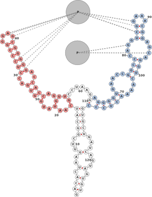
1.5 Kissing Hairpins
One often needs to depict the interaction between two molecules. Figure 5 shows two
small molecules interacting via a kissing hairpin interaction. It should be noted that
this is difficult to display when the interactions are longer than a few nucleotides due
to the layout constraints. Nevertheless, for shorter interactions, adding artificial
links can provide an adequate view of where molecules interact. For this
example, the following fasta sequences were entered in the ’Add Molecule’
dialog:
                  >a

UCAAAUGAGCUACUCACGUAGCUCAUCCUU

>b

CGAUAUGAGCUACGUGAGUAGCUCAUUGGU
The secondary structures are automatically predicted using RNAfold. The basepair nearest the hairpin is artificially broken (using ’shift’-click), and extra links are added between nucleotides 13,14,15,16 and 14,15,16,17.
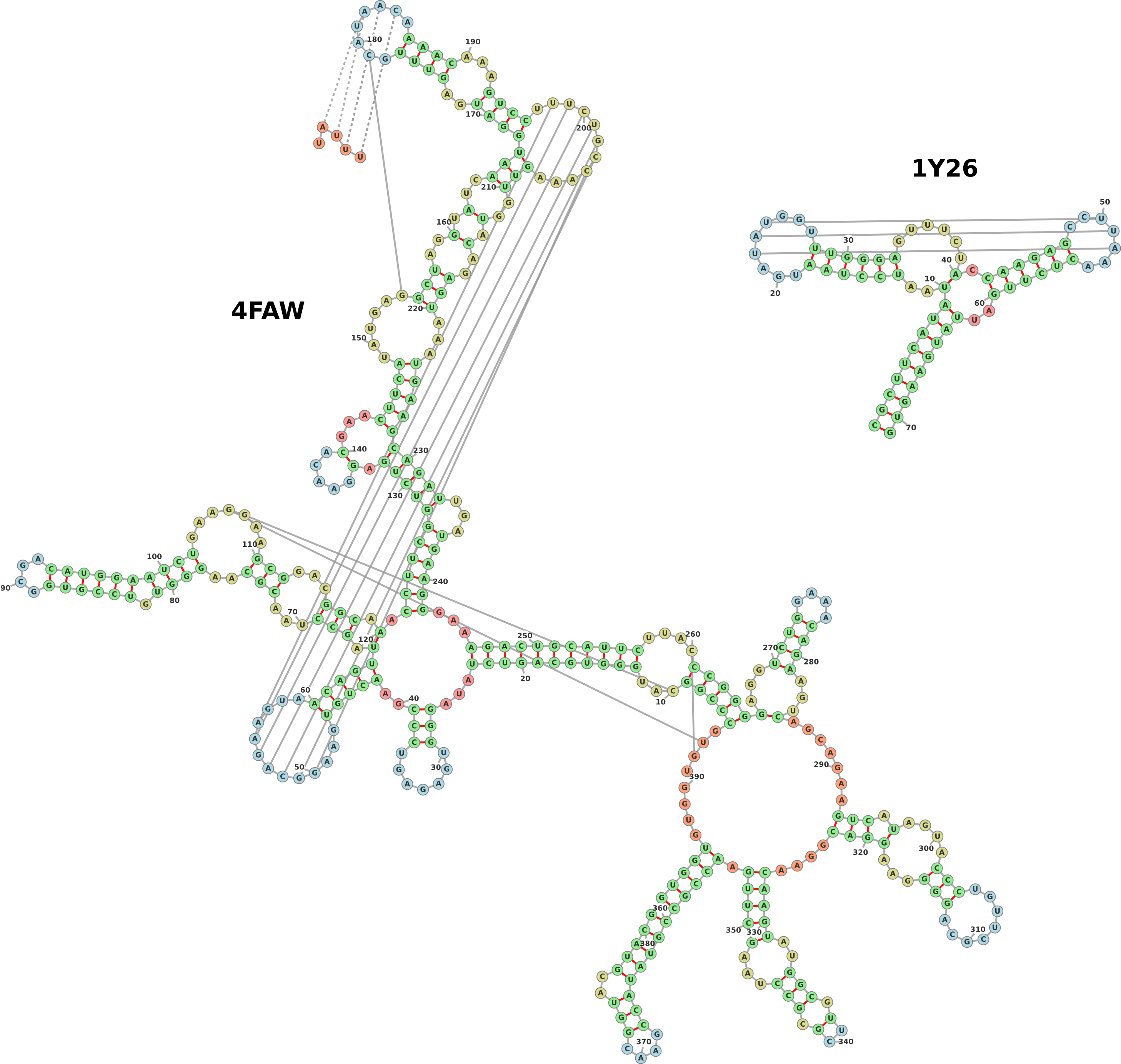
1.6 Pseudoknots
Pseudoknots are detected in the input structure using a greedy algorithm which
always marks the most nested base pairs as pseudoknots. These nested base pairs are
then added as strength-less links and removed from the rest of the structure. Figure 6
shows two examples of structures with pseudoknots, one input as a pdb file (group II
intron, PDB ID: 4FAW, left) and the other input from a dotbracket representation
(corresponding to an adenine riboswitch). The dotbracket string for generating
the structure on the right is shown below. Note the two different types of
brackets used (’()’ and ’[]’) in order to denote nested nucleotides. Other
brackets such as ’{}’ and ’<>’ can also be used to denote multiply nested
pairs.
                  >molecule_name

CGCUUCAUAUAAUCCUAAUGAUAUGGUUUGGGAGUUUCUACCAAGAGCCUUAAACUCUUGAUUAUGAAGUG

((((((((((..((((((...[[[...))))))......).((((((..]]]..))))))..)))))))))
1.7 Circular RNA
RNA usually exists as a single strand with distinct 5’ and 3’ ends, but it can also be
found as a circular molecule. Such molecules have been ligated at their 5’
and 3’ ends and thus have no external loops. These can be displayed using
forna (Figure 7) by appending an asterisk to the end of the dot-bracket
string.
                  >circular_rna

CUGCUCCACGCAAGGAGGUGGACUUAAGCGGCUCAUCCGGGUCUGCGAUAUCCACUGCGCGG

UAUGCGCUCGCGAGUUCGAAUCUCGUCGCCAGUACACUGACUUCACUGGCGUGUCCGAGUGG

UUAGGCAA

..(((((((....(((((((((.....(((((((....))).))))....))))))((((..

...))))..(((((.......)))))(((((((...........)))))))..)))..))))

...)))..*
Citations
[1] Gendron,P., et al. (2001) Quantitative analysis of nucleic acid threedimensional structures. Journal of molecular biology, 308 (5), 919–936[2] M. Antczak, T. Zok, M. Popenda, P. Lukasiak, R.W. Adamiak, J. Blazewicz, M. Szachniuk. RNApdbee - a webserver to derive secondary structures from pdb files of knotted and unknotted RNAs, Nucleic Acids Research 42(W1), 2014, W368-W372 (doi:10.1093/nar/gku330).